Analyzing Code Churn with Clojure and Zoo

by Adam Tornhill, June 2015

I've been presenting and writing about software evolution for a couple of years now. The single most common question I get is about the tools I use. I never talked much about them because I consider the tools the least important part of my message; It's much more important that we change our view of software design. That's still true, but I do want to contribute more in the tool's space; This article is the first in, what I hope, will become a series of tool related writings. Since Clojure is my primary language these days we'll start there.

Clojure in combination with the powerful Incanter library is a great platform for data analysis. In this article we'll put Clojure to work as you learn to calculate and visualize code churn trends.

Code churn is a powerful predictor of post-release defects, but it's real power lies in visualizing trends in your development projects. The tool we'll create in this article lets you reverse engineer your true development process from code. While the main purpose is to provide a short tutorial on Incanter's Zoo library, you'll also learn how to analyze time series in general.

You need a basic fluency of Clojure to follow along. Incanter and Zoo will be introduced below. The code used in this article is available on my GitHub account. Let's get started!

What's Code Churn?

Code churn is the amount of code you change in your system. There are multiple ways of measuring churn, but the most common is to calculate the number of added/modified/removed lines of code.

Code churn as added and
removed lines of code

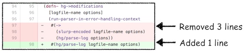
A single diff between two versions, as you see in the image above, is rarely that interesting; Instead we're after the trend. The kind of trend you want to calculate depends upon the questions you want to answer with your churn analysis. For example, in Your Code as a Crime Scene I describe several applications of a churn analysis:

Predict the modules with most defects.
Identify structural problems in your codebase.
Know where you need to focus extra test efforts.
Improve the workflow of your team
Predict when you'll be ~~done~~ DoneDone

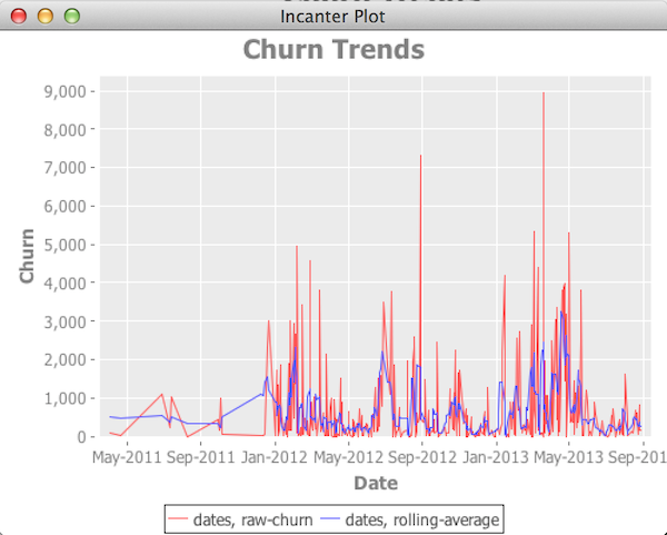
In this article we'll just focus on the last two points. The data we need, our target, looks something like the picture below:

Code
churn trends

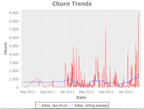
There are two lines in the picture. The red one shows the churn for each single day of the development project. The second line, the blue one, represents a rolling average. A rolling average is useful to smooth out fluctuations in the data and discover a possible overall trend.

In the picture above, we might be in for a problem; The trend shows a recent increase in churn. That's not a good sign if we're appraoching a deadline or a completion date since high code churn is correlated with post-release defects. A churn analysis gives you an early warning sign. But of course it all depends on context.

Now that we know where we're heading, let's see how we get the churn data that we need.

Show me the Tools

There are different kinds of churn metrics. If you want to predict defects you want to look into relative churn and have to analyze the code as well. For our purposes, however, we're only interested in the absolute churn values. That is, how many lines of code do we change each day? It's a question we can answer by version-control data alone.

I use Code Maat to mine the absolute churn metrics from a Git repository. Run Code Maat with the -a abs-churn argument to get a summary of the absolute churn. Here's what a typical output looks like:

        date,        added, deleted
        2011-04-04,    79,      8
        2011-04-20,    39,     27
        2011-06-28,  1116,    340
        2011-07-12,   214,     32
        2011-07-14,  1016,      0
        ...

Code Maat delivers all its output as CSV. The reason for that is because CSV is human readable, supported by spreadsheet applications, and easy to post-process.

Meet Incanter

Incanter is a set of libraries for statistical computing and visualizations. Incanter brings the power of the R-language to Clojure programmers. It's a powerful set of libraries, although sparingly documented. So let's see how we can put Incanter to work on our churn data.

Our first step is to reference the Incanter libraries that we'll use in our project.clj file:

        :dependencies [[org.clojure/clojure "1.6.0"]
	               [incanter "1.5.6"]
                       [incanter/incanter-zoo "1.5.6"]])

In this example we'll pull in the whole Incanter library just to keep it simple. It's important to note that you can pick just the parts you need instead (that's something you'd like to do in order to minimize the size of your executable program).

Now that we have specified the dependencies we need, let's fire up a REPL and get started:

        adam$ lein repl
        nREPL server started on port 51986 on host 127.0.0.1
        ...
        user=>

Read the raw data into a Dataset

To get the raw churn data into an Incanter dataset, we'll either pipe the output from Code Maat into our standard input stream or we persist the data to a file and read it from there.

Incanter has built-in support for reading CSV files. We just need to reference its IO package. Here's how it works:

         user=> (require '[incanter.io :as io])
         nil
         user=> (io/read-dataset "my_churn_data_from_code_maat.csv" :header true)

         |      :date | :added | :deleted |
         |------------+--------+----------|
         | 2011-04-04 |     79 |        8 |
         | 2011-04-20 |     39 |       27 |
         | 2011-06-28 |   1116 |      340 |
         ...

As you see, Incanter pretty prints the content of the created dataset. Let's run it one more time and bind the dataset to a var for further experimentation:

         user=> (def churn-ds (io/read-dataset "my_churn_data_from_code_maat.csv" :header true))
         #'user/churn-ds

Create a Zoo value to analyze time series

Remember, we want to track how our code churn changes over time. Incanter includes the Zoo library that makes it easy for us to work with such time series (Zoo is a port of the R Zoo package).

To do anything with Incanter Zoo, we have to convert our dataset into a Zoo value. That probably sounds more fancy than it is; A Zoo value is just a plain Incanter dataset that includes an index column of the time values.

Let's make a Zoo value out of our dataset:

         user=> (require '[incanter.zoo :as zoo])
         nil
         user=> (def churn-series (zoo/zoo churn-ds :date))
         #'user/churn-series

As you see in the code above, we just pass our dataset to the zoo function and specify the column in the dataset containing the dates (the :date column).

The Zoo conversion works out of the box because our original date format (yyyy-MM-dd) is coercible into Joda objects, which is what Zoo uses to populate its index column.

Now that we have a Zoo object, let's move on to more interesting algorithms and calculate a rolling average.

Calculate a rolling average to discover trends

Our Zoo dataset includes two different churn values, :deleted and :added:

         user=> churn-series
         
         |                   :index | :deleted | :added |
         |--------------------------+----------+--------|
         | 2011-04-04T00:00:00.000Z |        8 |     79 |
         | 2011-04-20T00:00:00.000Z |       27 |     39 |
         | 2011-06-28T00:00:00.000Z |      340 |   1116 |

In this example we'll just use calculate the trend for the positive churn, but you may want to play around with adding a trend for :deleted as well (it's straightforward).

To calculate a rolling average, we need to extract the data of interest from our dataset. Those functions are located in Incanter's core library so we need to require it first:

           user=> (require '[incanter.core :as i])

Here's the code for calculating our rolling average:

         (defn as-rolling-added-churn
          "Calculates a rolling average of the
           positive churn (added lines of code)."
           [ds n-days]
             (->>
              (i/sel ds :cols :added)
              (zoo/roll-mean n-days)
              (i/dataset [:rolling-added])
              (i/conj-cols ds)))

This algorithm first selects the values in the :added column from our dataset. Those values are threaded into Zoo's roll-mean function before we create a new single-column dataset of those mean values that we finally merge with the original Zoo dataset.

You probably noticed that we take a second argument, n-days, to our function. That parameter controls the sliding time window Zoo uses to calculate the rolling average. We'll get back to that value soon. Let's look at the resulting dataset first:

         user=> (as-rolling-added-churn churn-series 5)
         
         |                   :index | :deleted | :added | :rolling-added |
         |--------------------------+----------+--------+----------------|
         | 2011-04-04T00:00:00.000Z |        8 |     79 |         2464/5 |
         | 2011-04-20T00:00:00.000Z |       27 |     39 |         2388/5 |
         | 2011-06-28T00:00:00.000Z |      340 |   1116 |         2796/5 |
         ...

That looks just as we expected - all the data from the original dataset is there. In addition, we got the new column :rolling-added specifying the rolling average over 5 days.

Chose a meaningful sliding window

Zoo uses our provided n-days value to calculate the rolling average. Basically, the algorithm pics a subset of the data, calculates an average, and moves the time window ahead to select a new subset. Rinse and repeat until the data is exhausted.

We don't have to care much about it since Zoo implements that algorithm. What we do have to care about is to specify a sensible sliding window size.

I recommend that you use a value that's meaningful in your context. For example, if you work in iterations of two weeks length, go for 14 days as your sliding window.

Visualize the trend

Alright, we got the data we need. Let's visualize it and see how easy it is for our pattern-loving brain to spot trends.

Incanter includes a charts library built around the Java library JFreeChart. To use Incanter's charts we need to load its charts library:

         user=> (require '[incanter.charts :as charts])

Incanter's charting library contains all the basic charts you'd expect: histograms, lines and bar charts, box plots and more. Since we're after a trend over time we'll use the time-series-plot.

There are a few tricky things to keep in mind. The first is that the construction function for a time-series-plot only accepts one data series. That's a problem since we want to visualize two trends: 1) the raw churn, and 2) its rolling average.

We'll work around this limitation by constructing our chart in two steps:

First we create the chart with the raw churn.
Then we add a line for the rolling average using Incanter's charts/add-lines function.

Of course we encapsulate those steps in a function:

         (defn- as-time-series-plot
           [dates raw-churn rolling-average]
           (let [chart (charts/time-series-plot
                 dates
                 raw-churn
                 :title "Churn Trends"
                 :y-label "Churn"
                 :x-label "Date"
                 :legend true)]
         (charts/add-lines chart dates rolling-average)))

Now we just need to invoke as-time-series-plot to obtain our chart. The function takes three arguments. raw-churn and rolling-average are the values from the respective columns in our Zoo dataset. That's straightforward.

But the first argument, dates, requires your attention. We already have our time series in our dataset. We'll use it as X-axis but with one twist: Zoo requires us to convert our Joda time objects into milliseconds since the epoch. We express that conversion and data extraction in another function:

         (defn as-churn-chart
           [ds]
           (let [dates (map #(.getMillis %) (i/$ :index ds))
                 raw-added (i/$ :added ds)
                 rolling-added (i/$ :rolling-added ds)]
             (as-time-series-plot dates raw-added rolling-added)))

Our as-churn-chart function just calls the Java method getMillis on all time objects in our Zoo dataset (remember, a Zoo dataset is something with time objects in an :index column). We use Incanter's $ shortcut to select the data in the columns of interest. Everything is then fed to the as-time-series-plot function we defined above.

View the Chart

Now we got all the building blocks we need. Oh, almost; To actually view a chart we need to use Incanter's view function from its core library. Let's try it out at the REPL:

         user=> (->
                  (as-rolling-added-churn churn-series 5)
                   as-churn-chart
                   i/view)

The code above calculates a rolling average with a sliding window of five days. Here's how it looks:

Code
churn with rolling average

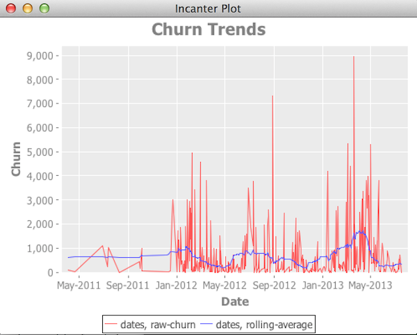
From here you can experiment with different sliding windows and look for possible long-term trends. For example, here's the rolling average over 30 days:

Code
churn with rolling
average of 30 days

I usually develop my Clojure code interactively like this in the REPL. Now that we have it all working, it's a good idea to package it up in named functions. So check out the sample code at my GitHub account for one approach.

Some closing words on Incanter

Incanter is powerful. It's also a huge API to learn. Fortunately, Incanter's design is fairly modular. So make sure to explore its different packages. Some are pretty specialized and you probably only need a few of them.

Another thing to keep in mind relates to application sizes. The strength of Incanter's modular design is that you only pay for what you use. Some of the libraries may be quite heavy to pull in so make sure you just specify the parts you really need in your project.clj file rather than the complete Incanter library. On my own projects I've cut the size of my executable jar files with half just by specifying the individual Incanter libraries individually.

That's it - I hope you've enjoyed our tour of code churn, datasets and Zoo!